Liebeskind Normal Mapping
Late last year, I had the idea of starting another game engine. My recent experiment with using Vulkan & Rust for a game jam left me in awe at the level of depth the Vulkan API offers. However, I was not a fan of Rust for engine development. The borrow checker in particular is made obsolete with patterns like the memory arena making memory leak a nonissue. So I set out to make a C++ and Vulkan engine, one that’ll keep me busy for years to come.
In graphics, two of the most fundamental techniques for encoding surface details are normal mapping and parallax occlusion mapping. I went ahead and implemented these first, and even made a presentation & live demo to Heavy Iron folks.
I heavily referenced LearnOpenGL’s tutorial on this topic, but figured I should make a writeup as a way to internalize my learning.
Normal Mapping
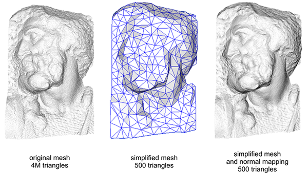 Back at school, I remember my graphics professor showing us a comparison between using
4 million triangles, and 500 but with normal mapping.
I was impressed at the similarities.
Back at school, I remember my graphics professor showing us a comparison between using
4 million triangles, and 500 but with normal mapping.
I was impressed at the similarities.
The technique involve encoding surface details in a texture instead of directly on the mesh, and saves a lot of memory and computation by texture interpolation.
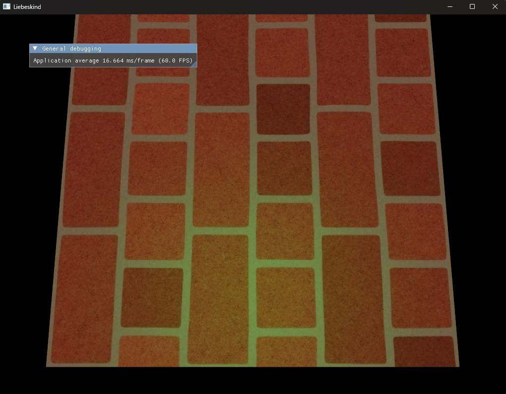
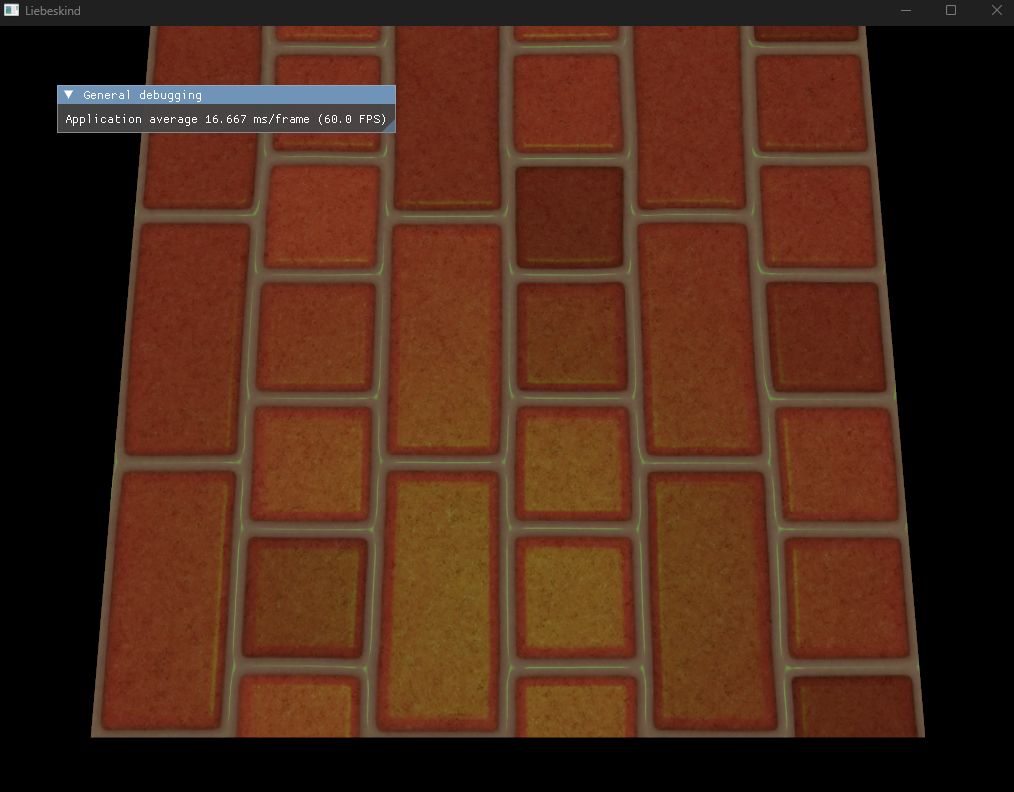
Applying this to a brick material in my engine Liebeskind yields a textured, elevated material even though both images below are flat quads.
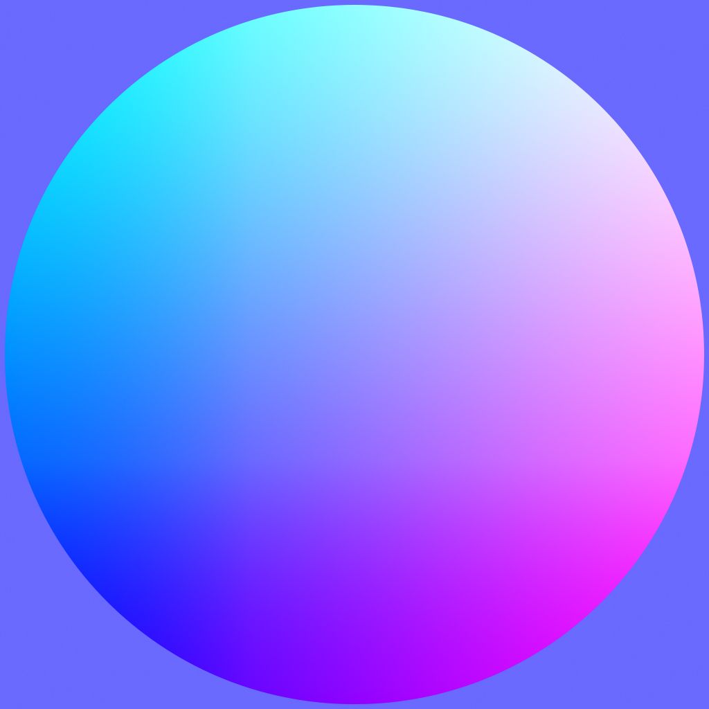 By convention, information is encoded into the red, green, and blue channel
of the normal map.
Each color correspond to a vector in the hemisphere formed by the surface and the
mesh normal.
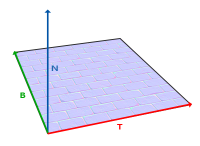
Typically, the tangent of the UV represents “right” in this hemisphere, and
bitangent up.
By convention, information is encoded into the red, green, and blue channel
of the normal map.
Each color correspond to a vector in the hemisphere formed by the surface and the
mesh normal.
Typically, the tangent of the UV represents “right” in this hemisphere, and
bitangent up.
You can transform a color value $\vec{c}$ in $[0,1]^3$ to a vector $\vec{v}$ in the hemisphere by \(\vec{v} = 2\vec{c} - 1\). Note that $\vec{v}$ here is not neccessarily a unit vector, and we’ll have to normalize this before we can use it in the fragment shader.
Tangent Space
 To even begin using a normal map, we need the tangent space at every fragment.
This is the space formed by the tangent (x), bitangent (y), and normal (z) of the surface.
Suppose we have a normal $\hat{N}$ for our surface.
There can be an infinite amount of (tangent, bitangent) pairs we can choose to form our tangent space.
Again, by convention, we choose tangent in the direction of increasing $u$ in UV space,
and bitangent in the direction of increasing $v$.
To even begin using a normal map, we need the tangent space at every fragment.
This is the space formed by the tangent (x), bitangent (y), and normal (z) of the surface.
Suppose we have a normal $\hat{N}$ for our surface.
There can be an infinite amount of (tangent, bitangent) pairs we can choose to form our tangent space.
Again, by convention, we choose tangent in the direction of increasing $u$ in UV space,
and bitangent in the direction of increasing $v$.
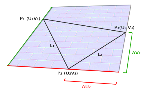 Imaging our mesh triangle mapped in UV space.
In practice, it will not lie on the edge of the UV space like the image, but can be any triangle in the space.
We get a system of linear equations for the values of $E_1$ and $E_2$:
Imaging our mesh triangle mapped in UV space.
In practice, it will not lie on the edge of the UV space like the image, but can be any triangle in the space.
We get a system of linear equations for the values of $E_1$ and $E_2$:
Where $\Delta U_1$ denotes the change in u value from $P_2$ to $P_1$, and $\Delta V_1$ denotes the change in v from $P_2$ to $P_3$. Now we can solve for the value of $T$ and $B$ using these.
\[\begin{align} \left[ \begin{array}{ccc} E_{1x} & E_{1y} & E_{1z}\\ E_{2x} & E_{2y} & E_{2z} \end{array} \right] &= \left[ \begin{array}{cc} U_1 & V_1 \\ U_2 & V_2 \end{array} \right] \left[ \begin{array}{ccc} T_{x} & T_{y} & T_{z}\\ B_{x} & B_{y} & B_{z} \end{array} \right] \end{align}\] \[\begin{align} \left[ \begin{array}{cc} U_1 & V_1 \\ U_2 & V_2 \end{array} \right]^{-1} \left[ \begin{array}{ccc} E_{1x} & E_{1y} & E_{1z}\\ E_{2x} & E_{2y} & E_{2z} \end{array} \right] &= \left[ \begin{array}{ccc} T_{x} & T_{y} & T_{z}\\ B_{x} & B_{y} & B_{z} \end{array} \right] \end{align}\] \[\begin{align} \frac{1}{det( \left[ \begin{array}{cc} U_1 & V_1 \\ U_2 & V_2 \end{array} \right] )} \left[ \begin{array}{cc} V_2 & -V_1 \\ -U_2 & U_1 \end{array} \right] \left[ \begin{array}{ccc} E_{1x} & E_{1y} & E_{1z}\\ E_{2x} & E_{2y} & E_{2z} \end{array} \right] &= \left[ \begin{array}{ccc} T_{x} & T_{y} & T_{z}\\ B_{x} & B_{y} & B_{z} \end{array} \right] \end{align}\] \[\begin{align} \frac{1}{U_1 V_2 - U_2 V_1} \left[ \begin{array}{cc} V_2 & -V_1 \\ -U_2 & U_1 \end{array} \right] \left[ \begin{array}{ccc} E_{1x} & E_{1y} & E_{1z}\\ E_{2x} & E_{2y} & E_{2z} \end{array} \right] &= \left[ \begin{array}{ccc} T_{x} & T_{y} & T_{z}\\ B_{x} & B_{y} & B_{z} \end{array} \right] \end{align}\]We only need to propagate the tangent to the vertex shader, since it’s possible to figure out what the bitangent is from that and the normal vector. So this is what our vertex input is:
struct Vertex {
    glm::vec3 position;
    glm::vec3 normal;
    glm::vec3 tangent;
    glm::vec3 color;
    glm::vec2 texCoord;
};
Now our vertex might be touching a lot of triangles, not just one. I choose to simply aggregate the tangents of all triangles touching a vertex, then normalize at the end. This is similar to how you would average normals of all touching faces to smooth out a corner.
constexpr int NUM_OF_VERTS_PER_TRIANGLE = 3;

for (int i = indexBegin; i < indices.size(); i += NUM_OF_VERTS_PER_TRIANGLE) {
	Vertex& v0 = vertices[indices[i]];
	Vertex& v1 = vertices[indices[i + 1]];
	Vertex& v2 = vertices[indices[i + 2]];

	glm::vec3 edge01 = v1.position - v0.position;
	glm::vec3 edge02 = v2.position - v0.position;

	glm::vec2 deltaUV01 = v1.texCoord - v0.texCoord;
	glm::vec2 deltaUV02 = v2.texCoord - v0.texCoord;

	float normalizer = 1.0f / (deltaUV01.x * deltaUV02.y -
							   deltaUV01.y * deltaUV02.x);

	glm::vec3 tangent =
		(deltaUV02.y * edge01 - deltaUV01.y * edge02) * normalizer;

	for (int k = 0; k < NUM_OF_VERTS_PER_TRIANGLE; k++)
		vertices[indices[i + k]].tangent += tangent;
}
Vertex Shader
Many, including the tutorial writer at LearnOpenGL, recommends transferring all outputs of the vertex shader to tangent space. This way, computing lighting is quite straightforward (since lighting is easiest done in tangent space). However, I choose to keep it in world space, since we can do more world space effects later down the line. This means piping the normal and tangent vectors from the vertex shader to the fragment shader:
normalWorld = vec3(transpose(inverse(transform)) * vec4(inNormal, 0.0));
tangentWorld = vec3(transform * vec4(inTangent, 0.0));
Fragment shader
The next part of normal mapping is literally doing the normal mapping. It involves
- calculating the tangent space in the fragment shader
- sampling the normal from the normal map and (3) using that normal for all lighting calculations.
One might be tempted to do the following:
bitangent = cross(inNormal, inTangent);
and while this sort of work, it will look wonky.
This is because the parameters at a fragment is an interpolated version of the parameter in neighboring vertices.
Therefore, it’s not guaranteed for inNormal or inTangent to be unit vectors, nor even orthogonal to each other.
We need to normalize these values and cancels out the projection of inNormal on inTangent:
void calculateTangentSpace() {
    normalWorld = normalize(inNormalWorld);
    tangentWorld = normalize(inTangentWorld - dot(inTangentWorld, normalWorld)
        * normalWorld);
    bitangentWorld = cross(normalWorld, tangentWorld);

    tangentToWorld = mat3(tangentWorld, bitangentWorld, normalWorld);
    // we can use transpose instead of inverse since the matrix is orthogonal
    worldToTangent = transpose(tangentToWorld);
}
Now we can use the normal map:
vec3 sampledNormalTangent = 2 * texture(normalSampler, inFragTexCoord).xyz - 1;
vec3 sampledNormalWorld = normalize(tangentToWorld * sampledNormalTangent);